Use Cases
Theory Predictions and their Uncertainties
EOS can produce theory predictions for any of its built-in observables.
The examples following in this section illustrate how to find a specific observable from the list of all built-in observables,
construct an Observable object and evaluate it,
and estimate the theoretical uncertainties associated with it.
Note
The following examples are intended to be run in an interactive Jupyter notebook. The entire notebook can be obtained from here.
Listing the built-in Observables
The full list of built-in observables for the most-recent EOS release is available online here. For an interactive approach to see the list of observables available to you, run the following in a Jupyter notebook
import eos
display(eos.Observables())
Searching for a specific observable is possible by filtering for specific strings in the observable name’s prefix, name, or suffix parts. The following example only shows observables that contain a ‘A_FB’ in the name part, and ‘B->pi in the prefix part, and ‘Untagged’ in the suffix part.
display(eos.Observables(name='A_FB'))
display(eos.Observables(prefix='B->pi'))
display(eos.Observables(suffix='Untagged'))
Constructing and Evaluating an Observable
To make theory predictions of any observable, EOS requires its full name, its Parameters object,
its Kinematics object, and its Options object.
As an example, we will use the integrated branching ratio of \(\bar{B}\to D\ell^-\bar\nu\),
which is represented by the QualifiedName B->Dlnu::BR.
Additional information about any given observable can be obtained by displaying the full database entry,
which also contains information about the kinematic variables required:
display(eos.Observables()['B->Dlnu::BR'])
which outputs the following table:
Qualified Name |
|
Description |
\(\mathcal{B}(\bar{B}\to D\ell^-\bar\nu)\) |
Kinematic Variable |
|
From this output we understand that B->Dlnu::BR expects two kinematic variables,
corresponding here to the lower and upper integration boundaries of the dilepton invariant mass \(q^2\).
We proceed to create an Obervable object with the default set of parameters and options,
and then display it:
params = eos.Parameters.Defaults()
kinematics = eos.Kinematics(q2_min=0.02, q2_max=10)
obs = eos.Observable.make('B->Dlnu::BR', params, kinematics, eos.Options())
display(obs)
The default options select \(\ell=\mu\) as the lepton flavor. The value of the observable is shown to be about \(2.4\%\), which is compatible with the current world average for the \(\bar{B}^-\to D^0\mu^-\bar\nu\) branching ratio.
By setting the l option to the value 'tau', we have create a different observable representing the \(\bar{B}^-\to D^0\tau^-\bar\nu\) branching ratio.
parameters = eos.Parameters.Defaults()
kinematics = eos.Kinematics(q2_min=3.17, q2_max=11.60)
obs = eos.Observable.make('B->Dlnu::BR', parameters, kinematics, eos.Options(l='tau'))
display(obs)
The new observable yields a value of \(0.69\%\).
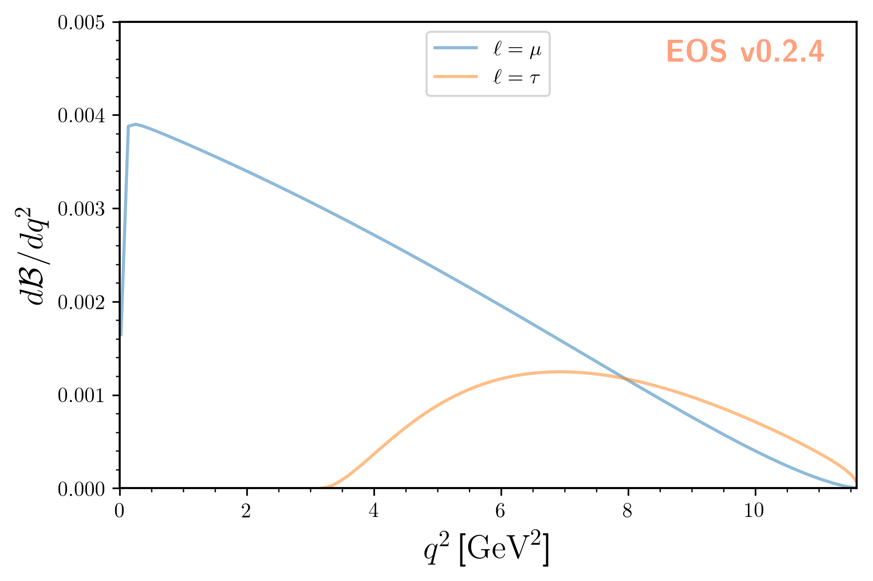
So far we evaluated the integrated branching ratio. EOS also provides the corresponding differential branching ratio
as a function of the squared momentum transfer \(q^2\).
The differential branching fraction is accessible through the name B->Dlnu::dBR/dq2. To illustrate it, we use EOS’s plot functions:
plot_args = {
    'plot': {
        'x': { 'label': r'$q^2$', 'unit': r'$\textnormal{GeV}^2$', 'range': [0.0, 11.60] },
        'y': { 'label': r'$d\mathcal{B}/dq^2$',                    'range': [0.0,  5e-3] },
        'legend': { 'location': 'upper center' }
    },
    'contents': [
        {
            'label': r'$\ell=\mu$',
            'type': 'observable',
            'observable': 'B->Dlnu::dBR/dq2;l=mu',
            'kinematic': 'q2',
            'range': [0.02, 11.60],
        },
        {
            'label': r'$\ell=\tau$',
            'type': 'observable',
            'observable': 'B->Dlnu::dBR/dq2;l=tau',
            'kinematic': 'q2',
            'range': [3.17, 11.60],
        }
    ]
}
eos.plot.Plotter(plot_args).plot()
which yields:
Estimating Theoretical Uncertainties
To estimate theoretical uncertainties of the observables, EOS uses Bayesian statistics. The latter interprets the theory parameters as random variables and assigns a priori probability density functions (prior PDFs) for each parameter.
Note
For technical reasons, EOS can only use uncorrelated prior PDFs. The same effects as having correlated prior PDFs can be achieved by using a correlated likelihood and uniform prior PDFs.
We carry on using the integrated branching ratios of \(\bar{B}^-\to D^0\left\lbrace\mu^-, \tau^-\right\rbrace\bar\nu\) decays as examples.
The largest source of theoretical uncertainty in these decays arises from the hadronic matrix elements, i.e.,
from the form factors \(f^{B\to \bar{D}}_+(q^2)\) and \(f^{B\to \bar{D}}_0(q^2)\).
Both form factors have been obtained independently using lattice QCD simulations by the HPQCD and Fermilab/MILC (FNAL+MILC) collaborations.
The joint likelihoods for both form factors at different \(q^2\) values of each prediction are available in EOS
as Constraint objects under the names B->D::f_++f_0@HPQCD:2015A and B->D::f_++f_0@FNAL+MILC:2015B.
We will discuss such constraints in more detail in the section Parameter Inference.
For this example, we will use both the HPQCD and FNAL+MILC results and create a combined likelihood as follows:
analysis_args = {
    'global_options': None,
    'priors': [
        { 'parameter': 'B->D::alpha^f+_0@BSZ2015', 'min':  0.0, 'max':  1.0, 'type': 'uniform' },
        { 'parameter': 'B->D::alpha^f+_1@BSZ2015', 'min': -5.0, 'max': +5.0, 'type': 'uniform' },
        { 'parameter': 'B->D::alpha^f+_2@BSZ2015', 'min': -5.0, 'max': +5.0, 'type': 'uniform' },
        { 'parameter': 'B->D::alpha^f0_1@BSZ2015', 'min': -5.0, 'max': +5.0, 'type': 'uniform' },
        { 'parameter': 'B->D::alpha^f0_2@BSZ2015', 'min': -5.0, 'max': +5.0, 'type': 'uniform' }
    ],
    'likelihood': [
        'B->D::f_++f_0@HPQCD:2015A',
        'B->D::f_++f_0@FNAL+MILC:2015B'
    ]
}
analysis = eos.Analysis(**analysis_args)
Next we create three observables: the semi-muonic branching ratio, the semi-tauonic branching ratio,
and the ratio of the former two. By using analysis.parameter in the construction of these
observables, we ensure that all observables and the Analysis object share the same parameter set.
This means that changes to the Analysis’ parameters will affect the evaluation
of all three observables.
obs_mu  = eos.Observable.make(
    'B->Dlnu::BR',
    analysis.parameters,
    eos.Kinematics(q2_min=0.02, q2_max=11.60),
    eos.Options(**{'l':'mu', 'form-factors':'BSZ2015'})
)
obs_tau = eos.Observable.make(
    'B->Dlnu::BR',
    analysis.parameters,
    eos.Kinematics(q2_min=3.17, q2_max=11.60),
    eos.Options(**{'l':'tau','form-factors':'BSZ2015'})
)
obs_R_D = eos.Observable.make(
    'B->Dlnu::R_D',
    analysis.parameters,
    eos.Kinematics(q2_mu_min=0.02, q2_mu_max=11.60, q2_tau_min=3.17, q2_tau_max=11.60),
    eos.Options(**{'form-factors':'BSZ2015'})
)
observables=(obs_mu, obs_tau, obs_R_D)
In the above, we made sure to provide the option form-factors=BSZ2015 to ensure that the right form factor plugin is used.
Sampling from the log(posterior) and – at the same time – producing posterior-predictive samples of the observables is achieved by running:
parameter_samples, log_weights, observable_samples = analysis.sample(N=5000, pre_N=1000, observables=observables)
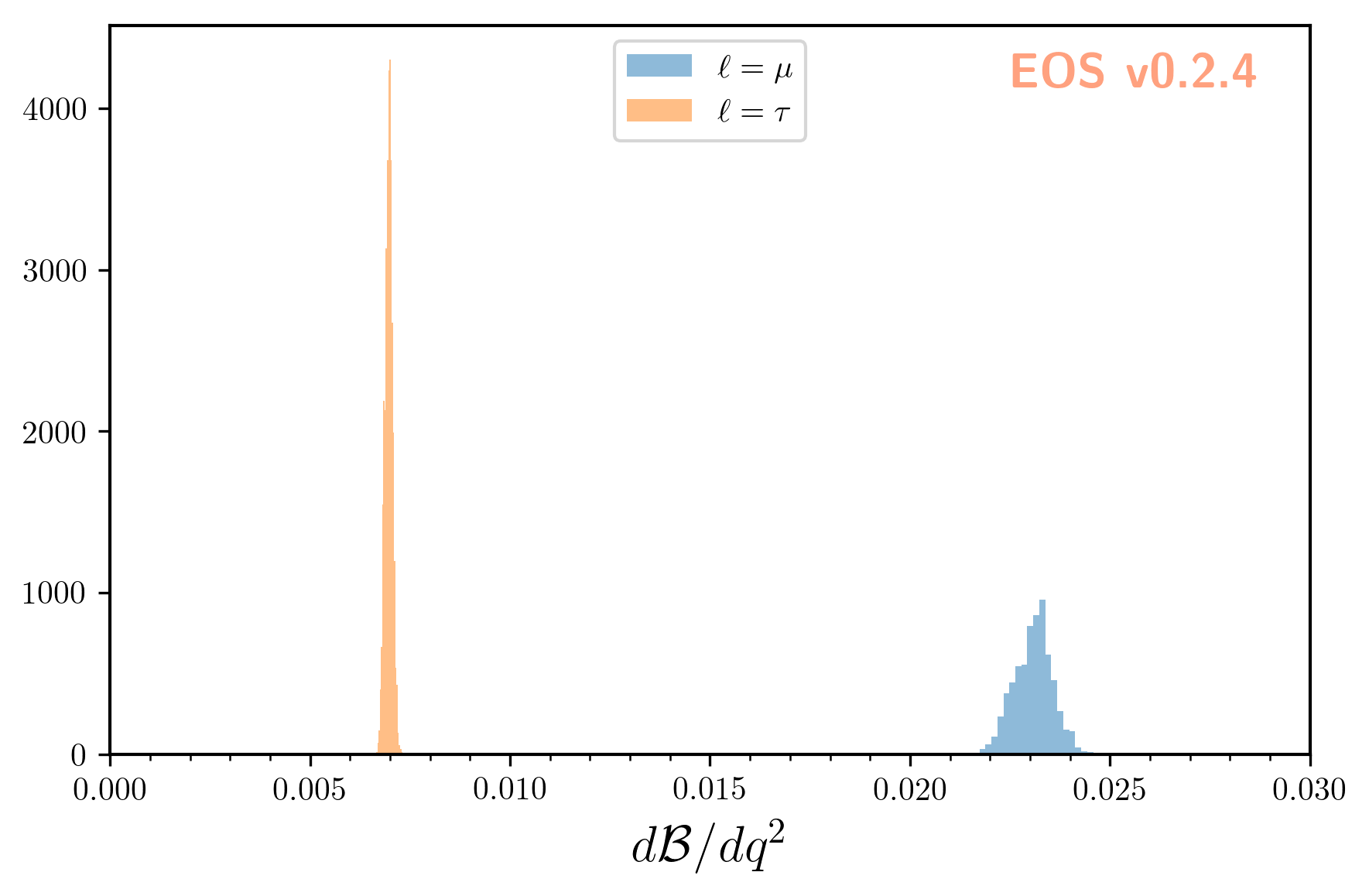
Here N=5000 samples are produced. To illustrate these samples we use EOS’ plotting framework:
plot_args = {
    'plot': {
        'x': { 'label': r'$d\mathcal{B}/dq^2$',  'range': [0.0,  3e-2] },
        'legend': { 'location': 'upper center' }
    },
    'contents': [
        { 'label': r'$\ell=\mu$', 'type': 'histogram', 'bins': 30, 'data': { 'samples': observable_samples[:, 0], 'log_weights': log_weights }},
        { 'label': r'$\ell=\tau$','type': 'histogram', 'bins': 30, 'data': { 'samples': observable_samples[:, 1], 'log_weights': log_weights }},
    ]
}
eos.plot.Plotter(plot_args).plot()
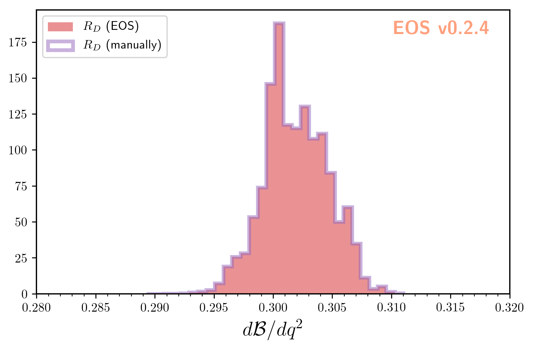
We can convince ourselves of the usefullness of the correlated samples by computing the lepton-flavor universality
ratio \(R_D\) twice: once using EOS’ built-in observable B->Dlnu::R_D as sampled above,
and once by calculating the ratio manually for each sample:
plot_args = {
    'plot': {
        'x': { 'label': r'$d\mathcal{B}/dq^2$',  'range': [0.28,  0.32] },
        'legend': { 'location': 'upper left' }
    },
    'contents': [
        { 'label': r'$R_D$ (EOS)',     'type': 'histogram', 'bins': 30, 'color': 'C3', 'data': { 'samples': observable_samples[:, 2] }},
        { 'label': r'$R_D$ (manually)','type': 'histogram', 'bins': 30, 'color': 'C4', 'data': { 'samples': [o[1] / o[0] for o in observable_samples[:]] },
          'histtype': 'step'},
    ]
}
eos.plot.Plotter(plot_args).plot()
Using the Numpy routines numpy.average and numpy.var we can produce numerical estimates
of the mean and the standard deviation:
import numpy as np
print('{obs};{opt}  = {mean:.4f} +/- {std:.4f}'.format(
    obs=obs_mu.name(), opt=obs_mu.options(),
    mean=np.average(observable_samples[:,0], weights=np.exp(log_weights)),
    std=np.sqrt(np.var(observable_samples[:, 0]))
))
print('{obs};{opt} = {mean:.4f} +/- {std:.4f}'.format(
    obs=obs_tau.name(), opt=obs_tau.options(),
    mean=np.average(observable_samples[:,1], weights=np.exp(log_weights)),
    std=np.sqrt(np.var(observable_samples[:, 1]))
))
print('{obs};{opt}      = {mean:.4f} +/- {std:.4f}'.format(
    obs=obs_R_D.name(), opt=obs_R_D.options(),
    mean=np.average(observable_samples[:,2], weights=np.exp(log_weights)),
    std=np.sqrt(np.var(observable_samples[:, 1]))
))
From the above we obtain:
B->Dlnu::BR;form-factors=BSZ2015,l=mu  = 0.0235 +/- 0.0007
B->Dlnu::BR;form-factors=BSZ2015,l=tau = 0.0071 +/- 0.0001
B->Dlnu::R_D;form-factors=BSZ2015      = 0.3014 +/- 0.0001
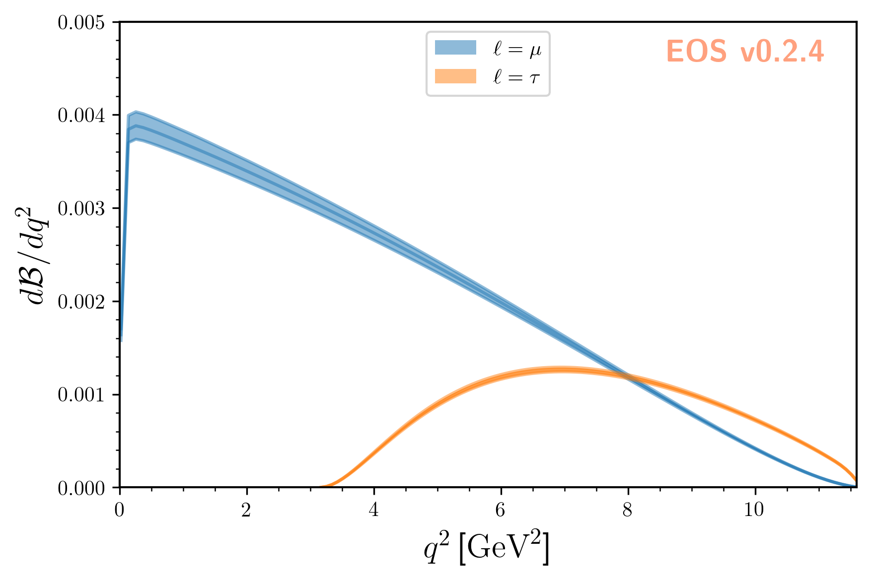
To obtain uncertainty bands for a plot of the differential branching ratios, we can now produce a
sequence of observables at different points in phase space. We then pass these observables on to
sample, to obtain posterior-predictive samples:
mu_q2values  = np.unique(np.concatenate((np.linspace(0.02,  1.00, 20), np.linspace(1.00, 11.60, 20))))
mu_obs       = [eos.Observable.make(
                   'B->Dlnu::dBR/dq2', analysis.parameters, eos.Kinematics(q2=q2),
                   eos.Options(**{'form-factors': 'BSZ2015', 'l': 'mu'}))
               for q2 in mu_q2values]
tau_q2values = np.linspace(3.17, 11.60, 40)
tau_obs      = [eos.Observable.make(
                   'B->Dlnu::dBR/dq2', analysis.parameters, eos.Kinematics(q2=q2),
                   eos.Options(**{'form-factors': 'BSZ2015', 'l': 'tau'}))
               for q2 in tau_q2values]
_, log_weights, mu_samples  = analysis.sample(N=5000, pre_N=1000, observables=mu_obs)
_, log_weights, tau_samples = analysis.sample(N=5000, pre_N=1000, observables=tau_obs)
We can plot the so-obtained posterior-predictive samples with EOS’ plotting framework by running:
plot_args = {
    'plot': {
        'x': { 'label': r'$q^2$', 'unit': r'$\textnormal{GeV}^2$', 'range': [0.0, 11.60] },
        'y': { 'label': r'$d\mathcal{B}/dq^2$',                    'range': [0.0,  5e-3] },
        'legend': { 'location': 'upper center' }
    },
    'contents': [
        {
          'label': r'$\ell=\mu$', 'type': 'uncertainty', 'range': [0.02, 11.60],
          'data': { 'samples': mu_samples, 'xvalues': mu_q2values }
        },
        {
          'label': r'$\ell=\tau$','type': 'uncertainty', 'range': [3.17, 11.60],
          'data': { 'samples': tau_samples, 'xvalues': tau_q2values }
        },
    ]
}
eos.plot.Plotter(plot_args).plot()
Parameter Inference
EOS can infer parameters based on a database of experimental or theoretical constraints and its built-in observables.
The examples following in this section illustrate how to find a specific constraint from the list of all built-in constraints,
construct an Analysis object that represents the statistical analysis,
and infer mean value and standard deviation of a list of parameters through optimization or Monte Carlo methods.
Note
The following examples are intended to be run in an interactive Jupyter notebook. The entire notebook can be obtained from here.
Listing the built-in Constraints
The full list of built-in constraints for the most-recent EOS release is available online here. For an interactive approach to see the list of constraints available to you, run the following in a Jupyter notebook:
import eos
display(eos.Constraints())
Searching for a specific observable is possible by filtering for specific strings in the constraint name’s prefix, name, or suffix parts. The following example only show constraints that contain ‘B^0->D^+’ in the prefix part:
display(eos.Constraints(prefix='B^0->D^+'))
Visualizing the built-in Constraints
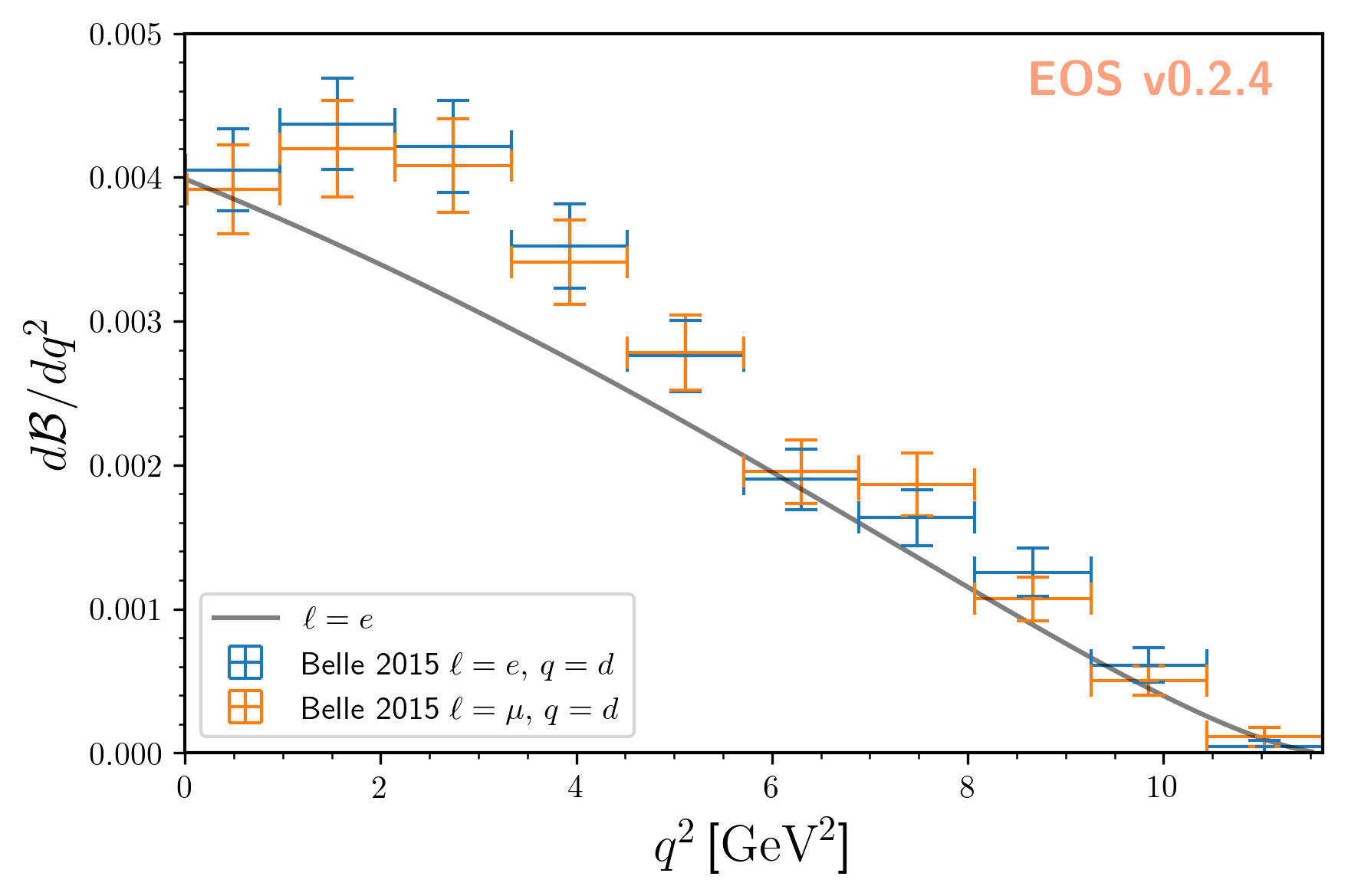
For what follows we will use the two experimental constraints B^0->D^+e^-nu::BRs@Belle:2015A and B^0->D^+mu^-nu::BRs@Belle:2015A,
to infer the CKM matrix element \(|V_{cb}|\). We can readily display these two constraints, along with the default theory prediction,
using the following code:
plot_args = {
    'plot': {
        'x': { 'label': r'$q^2$', 'unit': r'$\textnormal{GeV}^2$', 'range': [0.0, 11.63] },
        'y': { 'label': r'$d\mathcal{B}/dq^2$',                    'range': [0.0,  5e-3] },
        'legend': { 'location': 'lower left' }
    },
    'contents': [
        {
            'label': r'$\ell=e$',
            'type': 'observable',
            'observable': 'B->Dlnu::dBR/dq2;l=e,q=d',
            'kinematic': 'q2',
            'color': 'black',
            'range': [0.02, 11.63],
        },
        {
            'label': r'Belle 2015 $\ell=e,\, q=d$',
            'type': 'constraint',
            'color': 'C0',
            'constraints': 'B^0->D^+e^-nu::BRs@Belle:2015A',
            'observable': 'B->Dlnu::BR',
            'variable': 'q2',
            'rescale-by-width': False
        },
        {
            'label': r'Belle 2015 $\ell=\mu,\,q=d$',
            'type': 'constraint',
            'color': 'C1',
            'constraints': 'B^0->D^+mu^-nu::BRs@Belle:2015A',
            'observable': 'B->Dlnu::BR',
            'variable': 'q2',
            'rescale-by-width': False
        },
    ]
}
eos.plot.Plotter(plot_args).plot()
The resulting plot looks like this:
Defining the Statistical Analysis
To define our statistical analysis for the inference of \(|V_{cb}|\) from \(\bar{B}\to D\ell^-\bar\nu\) branching ratios, some decisions are needed. First, we must decide how to parametrize the hadronic form factors that emerge in semileptonic \(\bar{B}\to D\) transitions. For what follows we will use the [BSZ:2015A] parametrization. Next, we must decide the theory input for the form factors. For what follows we will combine the correlated lattice QCD results published by the Fermilab/MILC and HPQCD collaborations in 2015.
We then create an Analysis object as follows:
analysis_args = {
    'global_options': { 'form-factors': 'BSZ2015', 'model': 'CKM' },
    'priors': [
        { 'parameter': 'CKM::abs(V_cb)',           'min':  38e-3, 'max':  45e-3, 'type': 'uniform'},
        { 'parameter': 'B->D::alpha^f+_0@BSZ2015', 'min':  0.0,   'max':  1.0,   'type': 'uniform'},
        { 'parameter': 'B->D::alpha^f+_1@BSZ2015', 'min': -4.0,   'max': -1.0,   'type': 'uniform'},
        { 'parameter': 'B->D::alpha^f+_2@BSZ2015', 'min': +4.0,   'max': +6.0,   'type': 'uniform'},
        { 'parameter': 'B->D::alpha^f0_1@BSZ2015', 'min': -1.0,   'max': +2.0,   'type': 'uniform'},
        { 'parameter': 'B->D::alpha^f0_2@BSZ2015', 'min': -2.0,   'max':  0.0,   'type': 'uniform'}
    ],
    'likelihood': [
        'B->D::f_++f_0@HPQCD:2015A',
        'B->D::f_++f_0@FNAL+MILC:2015B',
        'B^0->D^+e^-nu::BRs@Belle:2015A',
        'B^0->D^+mu^-nu::BRs@Belle:2015A'
    ]
}
analysis = eos.Analysis(**analysis_args)
analysis.parameters['CKM::abs(V_cb)'].set(42.0e-3)
In the above, the global options ensure that our choice of form factor parametrization is used throughout,
and that for CKM matrix elements the CKM model is used. The latter provides access to \(V_{cb}\) matrix element through two parameters:
the absolute value CKM::abs(V_cb) and the complex phase CKM::arg(V_cb).
We provide the parameters in our analysis through the specifications of the Bayesian priors.
In the above, each prior is a uniform prior that covers the range from min to max.
The likelihood is defined through a list constraints, which in the above includes both the experimental measurements by the Belle collaboration as well as the theoretical lattice QCD results.
Finally, we set the starting value of CKM::abs(V_cb) to a sensible value of \(42\cdot 10^{-3}\).
We can now proceed to optimize the log(posterior) through a call to analysis.optimize.
In a Jupyter notebook, it is useful to display the return value of this method, which illustrates the best-fit point.
We can further display a summary of the goodness-of-fit information.
bfp = analysis.optimize()
display(bfp)
display(analysis.goodness_of_fit())
The resulting best-fit point looks like this:
parameter |
value |
\(|V_{cb}|\) |
0.0422 |
|
0.6671 |
|
-2.5314 |
|
4.8813 |
|
0.2660 |
|
-0.8410 |
The goodness-of-fit summary consists of a table listing all constraints,
constraint |
\(\chi^2\) |
d.o.f. |
|
3.4847 |
7 |
|
3.1016 |
5 |
|
11.8206 |
10 |
|
5.2242 |
10 |
and the overall information including the p value:
total \(\chi^2\) |
23.6310 |
total degrees of freedom |
26 |
p-value |
59.7053% |
Sampling from the Posterior
To sample from the posterior, EOS provides the sample method.
Optionally, this can also produce posterior-predictive samples for a list of observables.
We can use these samples to illustrate the results of our fit in relation to the experimental constraints.
For this example, we produce such posterior-predictive samples for the differential \(\bar{B}\to D^+e^-\bar\nu\) branching ratio in 40 points in the kinematical variable \(q^2\):; the square of the momentum transfer to the \(e^-\bar\nu\) pair. Due to the strong dependence of the branching ratio on \(q^2\), we do not distribute the points equally across the full phase space. Instead, we equally distribute half of the points in the interval \([0.02\,\text{GeV}^2, 1.00\,\text{GeV}^2]\) and the other half in the remainder of the phase space.
We run one Markov chain to produce N = 20000 samples with a thinning factor (or stride) of 5.
This means that stride * N = 100000 samples are produced, but only every 5th sample is returned.
This improves the quality of the samples by reducing the autocorrelation.
Before the samples are produced, the Markov Chain self-adapts in a series of preruns,
the number of which is governed by the preprun argument. In each prerun, pre_N
samples are drawn before the adaptation step. The samples obtained as part of the
preruns are discarded. To ensure efficient sampling, the chain is started in the
best-fit point obtained earlier through optimization.
e_q2values  = np.unique(np.concatenate((np.linspace(0.02,  1.00, 20), np.linspace(1.00, 11.60, 20))))
e_obs       = [eos.Observable.make(
                  'B->Dlnu::dBR/dq2', analysis.parameters, eos.Kinematics(q2=q2),
                  eos.Options(**{'form-factors': 'BSZ2015', 'l': 'e', 'q': 'd'}))
              for q2 in e_q2values]
parameter_samples, log_weights, e_samples  = analysis.sample(N=20000, stride=5, pre_N=1000, preruns=5, start_point=bfp.point, observables=e_obs)
The values of the log(posterior) are stored in log_posterior.
The posterior-preditive samples for the observables are stored in e_samples,
and are only returned if the observables keyword argument is provided.
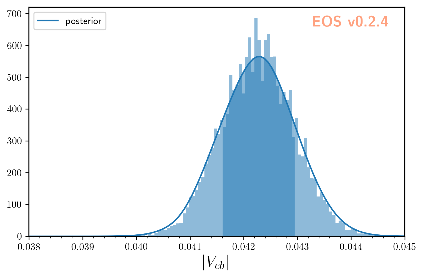
We can illustrate the posterior samples either as a histogram or as a kernel density estimate (KDE) using the built-in plotting functions:
plot_args = {
    'plot': {
        'x': { 'label': r'$|V_{cb}|$', 'range': [38e-3, 45e-3] },
        'legend': { 'location': 'upper left' }
    },
    'contents': [
        {
            'type': 'histogram',
            'data': { 'samples': parameter_samples[:, 0], 'log_weights': log_weights }
        },
        {
            'type': 'kde', 'color': 'C0', 'label': 'posterior', 'bandwidth': 2,
            'range': [40e-3, 45e-3],
            'data': { 'samples': parameter_samples[:, 0], 'log_weights': log_weights }
        }
    ]
}
eos.plot.Plotter(plot_args).plot()
The result looks like this:
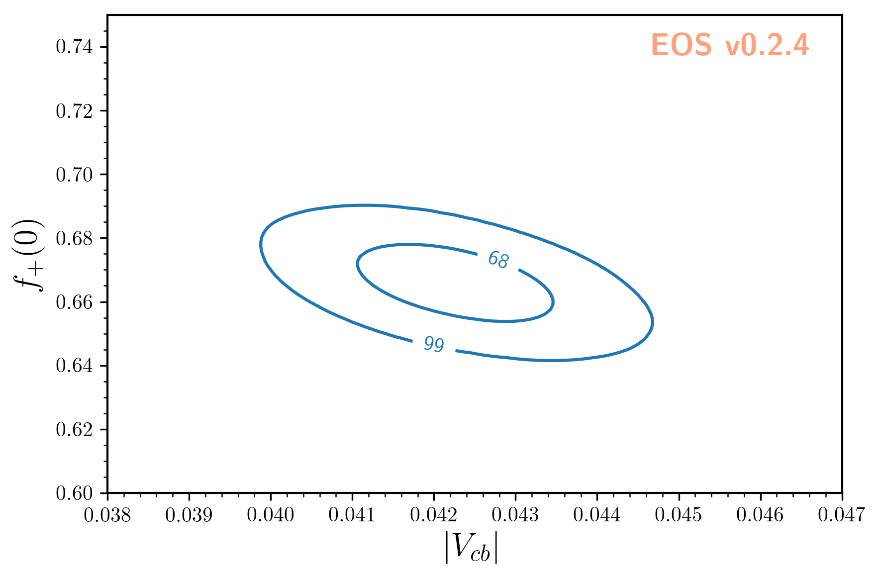
Contours at given levels of posterior probability can be obtained for any pair of parameters using:
plot_args = {
    'plot': {
        'x': { 'label': r'$|V_{cb}|$', 'range': [38e-3, 47e-3] },
        'y': { 'label': r'$f_+(0)$', 'range': [0.6, 0.75] },
    },
    'contents': [
        {
            'type': 'kde2D', 'color': 'C1', 'label': 'posterior',
            'range': [40e-3, 45e-3], 'levels': [68, 99], 'bandwidth': 3,
            'data': { 'samples': parameter_samples[:, (0,1)], 'log_weights': log_weights }
        }
    ]
}
eos.plot.Plotter(plot_args).plot()
The result looks like this:
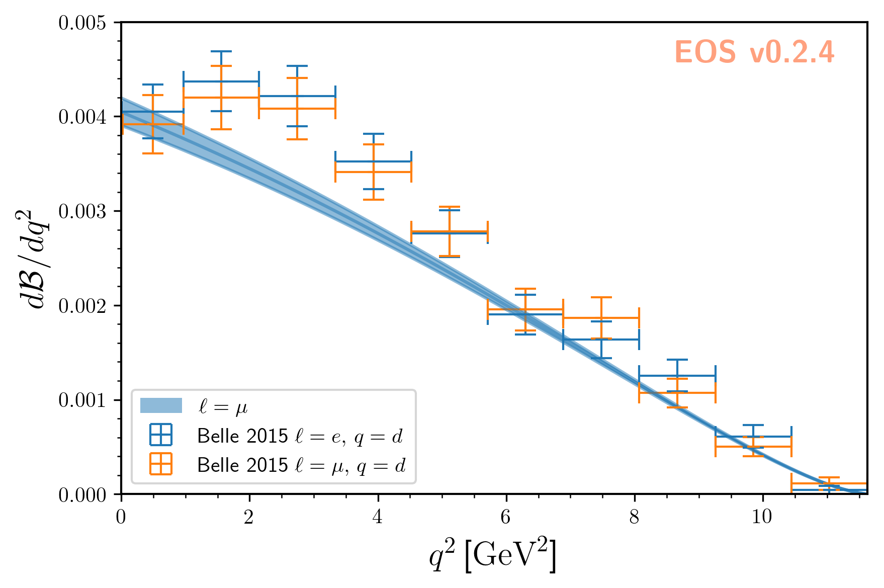
We can visualize the posterior-predictive samples using:
plot_args = {
    'plot': {
        'x': { 'label': r'$q^2$', 'unit': r'$\textnormal{GeV}^2$', 'range': [0.0, 11.63] },
        'y': { 'label': r'$d\mathcal{B}/dq^2$',                    'range': [0.0,  5e-3] },
        'legend': { 'location': 'lower left' }
    },
    'contents': [
        {
          'label': r'$\ell=\mu$', 'type': 'uncertainty', 'range': [0.02, 11.60],
          'data': { 'samples': e_samples, 'xvalues': e_q2values }
        },
        {
            'label': r'Belle 2015 $\ell=e,\, q=d$',
            'type': 'constraint',
            'color': 'C0',
            'constraints': 'B^0->D^+e^-nu::BRs@Belle:2015A',
            'observable': 'B->Dlnu::BR',
            'variable': 'q2',
            'rescale-by-width': False
        },
        {
            'label': r'Belle 2015 $\ell=\mu,\,q=d$',
            'type': 'constraint',
            'color': 'C1',
            'constraints': 'B^0->D^+mu^-nu::BRs@Belle:2015A',
            'observable': 'B->Dlnu::BR',
            'variable': 'q2',
            'rescale-by-width': False
        },
    ]
}
eos.plot.Plotter(plot_args).plot()
The result looks like this:
Pseudo Event Simulation
EOS can simulate pseudo events from any of its built-in PDFs using Markov chain Monte Carlo techniques. The examples following in this section illustrate how to find a specific PDF from the list of all built-in PDFs, simulate the pseudo events from this object, compare to the pseudo events with the analytic results, and plot 1D and 2D histograms of the pseudo events.
Note
The following examples are intended to be run in an interactive Jupyter notebook. The entire notebook can be obtained from here.
Listing the built-in Probability Density Functions
The full list of built-in PDFs for the most-recent EOS release is available online here. For an interactive approach to see the list of PDFs available to you, run the following in a Jupyter notebook:
import eos
display(eos.SignalPDFs())
Searching for a specific PDF is possible by filtering for specific strings in the PDF name’s prefix, name, or suffix parts. The following example only shows PDFs that contain ‘B->Dlnu’ in the prefix part.
display(eos.SignalPDFs(prefix='B->Dlnu'))
Constructing a 1D PDF and Simulating Pseudo Events
We construct the one-dimension PDF describing the decay distribution in the variable \(q^2\) and for \(\ell=\mu\) leptons.
We create the q2 kinematic variable and set it to an arbitrary starting value.
We set boundaries for the phase space from which we want to sample through the kinematic variables q2_min and q2_max.
If needed, we can shrink the phase space to a volume smaller than physically allowed. The normalization of the PDF will automatically adapt.
We simulate stride * N=250000 pseudo events/samples from the PDF, which are thinned down to N=50000.
The Markov chains can self adapt to the PDF in preruns=3 preruns with pre_N=1000 pseudo events/samples each.
mu_kinematics = eos.Kinematics(**{
    'q2':            2.0,  'q2_min':            0.02,     'q2_max':           11.6,
})
mu_pdf = eos.SignalPDF.make('B->Dlnu::dGamma/dq2', eos.Parameters(), mu_kinematics, eos.Options())
rng = np.random.mtrand.RandomState(74205)
mu_samples, mu_weights = mu_pdf.sample_mcmc(N=50000, stride=5, pre_N=1000, preruns=3, rng=rng)
We repeat the exercise for \(\ell=\tau\) leptons, and adapt the phase space accordingly.
tau_kinematics = eos.Kinematics(**{
    'q2':            4.0,  'q2_min':            3.17,     'q2_max':           11.6,
})
tau_pdf = eos.SignalPDF.make('B->Dlnu::dGamma/dq2', eos.Parameters(), tau_kinematics, eos.Options(l='tau'))
rng = np.random.mtrand.RandomState(74205)
tau_samples, tau_weights = tau_pdf.sample_mcmc(N=50000, stride=5, pre_N=1000, preruns=3, rng=rng)
Comparing the 1D PDF pseudo events with the analytic result
We can now histogram the pseudo events/samples and compare the histogram with the analytical result.
Similar to observables, SignalPDF objects can be plotted as a function of a single kinematic variable,
while keeping all other kinematic variables fixed. The latter is achieved via the kinematics key.
plot_args = {
    'plot': {
        'x': { 'label': r'$q^2$', 'unit': r'$\textnormal{GeV}^2$', 'range': [0.0, 11.60] },
        'y': { 'label': r'$P(q^2)$',                               'range': [0.0,  0.25] },
        'legend': { 'location': 'upper left' }
    },
    'contents': [
        {
            'label': r'samples ($\ell=\mu$)',
            'type': 'histogram',
            'data': {
                'samples': mu_samples
            },
            'color': 'C0'
        },
        {
            'label': r'samples ($\ell=\tau$)',
            'type': 'histogram',
            'data': {
                'samples': tau_samples
            },
            'color': 'C1'
        },
        {
            'label': r'PDF ($\ell=\mu$)',
            'type': 'signal-pdf',
            'pdf': 'B->Dlnu::dGamma/dq2;l=mu',
            'kinematic': 'q2',
            'range': [0.02, 11.60],
            'kinematics': {
                'q2_min':  0.02,
                'q2_max': 11.60,
            },
            'color': 'C0'
        },
        {
            'label': r'PDF ($\ell=\tau$)',
            'type': 'signal-pdf',
            'pdf': 'B->Dlnu::dGamma/dq2;l=tau',
            'kinematic': 'q2',
            'range': [3.17, 11.60],
            'kinematics': {
                'q2_min':  3.17,
                'q2_max': 11.60,
            },
            'color': 'C1'
        },
    ]
}
eos.plot.Plotter(plot_args).plot()
The result looks like this:

As you can see, we have excellent agreement between our simulations and the respective analytic expressions for the PDFs.
Constructing a 4D PDF and Simulating Pseudo Events
We can also draw samples for PDFs with more than two kinematic variables. Here, we use the full four-dimensional PDF for \(\bar{B}\to D^*\ell^-\bar\nu\) decays.
We declare and initialize all four kinematic variables (q2, cos(theta_l), cos(theta_d), and phi),
and provide the phase space boundaries (same names appended with _min and _max).
We then produce the samples as for the 1D PDF.
dstarlnu_kinematics = eos.Kinematics(**{
    'q2':            2.0,  'q2_min':            0.02,     'q2_max':           10.5,
    'cos(theta_l)':  0.0,  'cos(theta_l)_min': -1.0,      'cos(theta_l)_max': +1.0,
    'cos(theta_d)':  0.0,  'cos(theta_d)_min': -1.0,      'cos(theta_d)_max': +1.0,
    'phi':           0.3,  'phi_min':           0.0,      'phi_max':           2.0 * np.pi
})
dstarlnu_pdf = eos.SignalPDF.make('B->D^*lnu::d^4Gamma', eos.Parameters(), dstarlnu_kinematics, eos.Options())
rng = np.random.mtrand.RandomState(74205)
dstarlnu_samples, _ = dstarlnu_pdf.sample_mcmc(N=50000, stride=5, pre_N=1000, preruns=3, rng=rng)
We can now show correlations of the kinematic variables by plotting 2D histograms, beginning with \(q^2\) vs \(\cos\theta_\ell\), …
plot_args = {
    'plot': {
        'x': { 'label': r'$q^2$', 'unit': r'$\textnormal{GeV}^2$', 'range': [ 0.0, 10.50] },
        'y': { 'label': r'$cos(\theta_\ell)$',                     'range': [-1.0,  +1.0] },
        'legend': { 'location': 'upper left' }
    },
    'contents': [
        {
            'label': r'samples ($\ell=\mu$)',
            'type': 'histogram2D',
            'data': {
                'samples': dstarlnu_samples[:, (0, 1)]
            },
            'bins': 40
        },
    ]
}
eos.plot.Plotter(plot_args).plot()
… over \(\cos\theta_\ell\) vs \(\cos\theta_D\) …
plot_args = {
    'plot': {
        'x': { 'label': r'$cos(\theta_\ell)$',                     'range': [-1.0,  +1.0] },
        'y': { 'label': r'$cos(\theta_D)$',                        'range': [-1.0,  +1.0] },
        'legend': { 'location': 'upper left' }
    },
    'contents': [
        {
            'label': r'samples ($\ell=\mu$)',
            'type': 'histogram2D',
            'data': {
                'samples': dstarlnu_samples[:, (1, 2)]
            },
            'bins': 40
        },
    ]
}
eos.plot.Plotter(plot_args).plot()
… to \(q^2\) vs \(\phi\).
plot_args = {
    'plot': {
        'x': { 'label': r'$q^2$', 'unit': r'$\textnormal{GeV}^2$', 'range': [0.0, 10.70] },
        'y': { 'label': r'$\phi$',                                 'range': [0.0,  6.28] },
        'legend': { 'location': 'upper left' }
    },
    'contents': [
        {
            'label': r'samples ($\ell=\mu$)',
            'type': 'histogram2D',
            'data': {
                'samples': dstarlnu_samples[:, (0, 3)]
            },
            'bins': 40
        },
    ]
}
eos.plot.Plotter(plot_args).plot()
The results look as follows:


