Analysis Organisation

This notebook illustrates how to organise your analysis or analyses. This presentation is based on the physical example of the analysis of \(b \to u \ell \nu\) exclusive decays. The analysis properties are encoded in a companion file named b-to-u-l-nu.yaml, which fully describes a number of individual priors and likelihoods. These objects serve as the building blocks to construct individual posteriors, which are then available for the overall analysis.

Defining the Building Blocks

The analysis file is loaded via eos.AnalysisFile. In our case the file defines two posteriors CKM-all and WET-all, and a few priors and likelihoods, which are used to define the two posteriors. The file format is YAML.

import eos
import os
from IPython.display import Markdown as md

af = eos.AnalysisFile('./b-to-u-l-nu.yaml')

[ObservableEntries.insert_or_assign] Entry for observable B->pilnu::R_pi has been replaced.

Defining parameters

The parametrization in EOS strives to be as specific as possible. Hence, EOS treats the Wilson coefficients as lepton flavor specific. To restore lepton flavor universality, we create a new set of lepton flavor universal parameters and alias the existing parameters for the lepton specific Wilson coefficients to the new set.

Looking at the b->u parameters available in EOS, we see that all available Wilson coefficients are lepton flavor dependent:

display(eos.Parameters(prefix='ub', name='Re{cVL}'))

qualified name	symbol	unit	value
Standard Model and Effective Field Theory Parameters
$\bar{u}b\bar{\ell}\nu$ WET Parameters
The list of parameters describing the Wilson coefficients of $\bar{u}b\bar{\ell}\nu$ operators in the effective Lagrangian \begin{equation} \mathcal{H}^{\bar{u}b\bar{\ell}\nu}_\mathrm{eff} = \frac{4 G_F}{\sqrt{2}} V_{ub} \sum_i \mathcal{C}^{\bar{u}b\bar{\ell}\nu}_i \mathcal{O}^{\bar{u}b\bar{\ell}\nu}_i\,. \end{equation} The operators read: \begin{align} \mathcal{O}_{V_{L(R)}} & = [\bar{u} \gamma^\mu P_{L(R)} b]\, [\bar{\ell} \gamma_\mu P_L \nu_\ell]\\ \mathcal{O}_{S_{L(R)}} & = [\bar{u} P_{L(R)} b]\, [\bar{\ell} P_L \nu_\ell]\\ \mathcal{O}_{T} & = [\bar{u} \sigma^{\mu\nu} b]\, [\bar{\ell} \sigma_{\mu\nu} P_L \nu_\ell] \end{align}
ubenue::Re{cVL}	$$\mathrm{Re}\, \mathcal{C}^{\bar{u}b\bar{e}\nu_e}_{V_L}$$	—	1.0
ubmunumu::Re{cVL}	$$\mathrm{Re}\, \mathcal{C}^{\bar{u}b\bar{\mu}\nu_\mu}_{V_L}$$	—	1.0
ubtaunutau::Re{cVL}	$$\mathrm{Re}\, \mathcal{C}^{\bar{u}b\bar{\tau}\nu_\tau}_{V_L}$$	—	1.0

Here we show how to define a new parameter which is an alias to all three lepton flavor dependent left-handed vector Wilson coefficients:

parameters:
  'ublnul::Re{cVL}' :
      alias_of: [ 'ubenue::Re{cVL}', 'ubmunumu::Re{cVL}', 'ubtaunutau::Re{cVL}' ]
      central:   1.0
      min:      -2.0
      max:       2.0
      unit:     '1'
      latex:    '$\mathrm{Re}\, \mathcal{C}^{\bar{u}b\bar{\nu}_\ell\ell}_{V_L}$'
  ...

The alias_of key is a list of existing EOS parameters (by qualified name). In the b-to-u-l-nu.yaml analysis file we similarly do so for scalar and tensor Wilson coefficients.

Defining priors

All priors are contained within a list associated with the top-level key priors. In the example, the WET prior is defined as follows:

priors:
  ...
    - name: WET
    descriptions:
      - { 'parameter': 'ublnul::Re{cVL}', 'min':  0.9, 'max': 1.2, 'type': 'uniform' }
      ...

The definition associates a list of all parameters varied as part of this prior with the key descriptions. Each element of the list is a dictionary representing a single parameter. It provides the parameter’s full name as parameter, lists the min/max interval, and specifies the type of prior distribution. This format reflects the expectations of the prior keyword argument of eos.Analysis.

In addition to the descriptions key one can also pass manual constraints via the manual_constraints key or pyhf constraints via the pyhf key.

Defining likelihoods

All likelihoods are contained within a list associated with the top-level key likelihoods. In the EOS convention, theoretical and experimental likelihoods should be defined separately from each other and their names prefixed with TH- and EXP-, respectively. In the example file, the TH-pi likelihoods is defined as follows:

likelihoods:
  - name: TH-pi
    constraints:
      - 'B->pi::form-factors[f_+,f_0,f_T]@LMvD:2021A;form-factors=BCL2008-4'
      - 'B->pi::f_++f_0+f_T@FNAL+MILC:2015C;form-factors=BCL2008-4'
      - 'B->pi::f_++f_0@RBC+UKQCD:2015A;form-factors=BCL2008-4'
  ...

The definition associates a list of constraints with the key constraints. Each element of the list is a string referring to one of the built-in EOS constraints. This format reflects the expectations of the constraints keyword argument of eos.Analysis.

Defining posteriors

We define a posterior based on predefined likelihoods and priors within a list associated with the top-level key posteriors as

posteriors:
  ...
  - name: WET-all
    global_options:
      model: WET
    fixed_parameters:
      CKM::abs(V_ub): 3.67e-3
    prior:
      - WET
      - DC-Bu
      - FF-pi
    likelihood:
      - TH-pi
      - EXP-pi
      - EXP-leptonic

The specification of global options ensures that we use the CKM model for CKM matrix elements and that we focus on electrons in our final state. Using the fixed_parameters key we fix \(|V_{ub}|\) here.

In the analysis file we add two posteriors, for the CKM model and the WET model. Below we sample from both posteriors.

Defining observables

By defining and using custom observables in this way, you can tailor your analysis to include specific quantities of interest and ensure that they are properly accounted for in your results. To define custom observables, one can add an entry to the observables part of the analysis file. Mandatory fields include the name of the observable, the latex expression, its unit and an expression for the observable. The expression is constructed as documented here.

observables:
  "B->pilnu::R_pi":
    latex: "$R_{\\pi}$"
    unit: '1'
    options: {}
    expression: "<<B->pilnu::BR;l=tau>>[q2_min=>q2_tau_min] / <<B->pilnu::BR;l=e>>[q2_min=>q2_e_min]"

Defining predictions

To finally produce posterior predictive distributions for some observables, we can add them via the predictions key:

predictions:
  - name: leptonic-BR-CKM
    global_options:
      model: CKM
    observables:
      - name: B_u->lnu::BR;l=e
      - name: B_u->lnu::BR;l=mu
      - name: B_u->lnu::BR;l=tau
  ...

Here we add the total branching ratio of \(\bar{B} \to \ell^- \bar{\nu}\) for \(l=e, \mu, \tau\) as prediction.

Similarly, we can add a prediction for our custom observable, defined above:

- name : R_pi
  global_options:
    model: WET
  observables:
    - name: B->pilnu::R_pi
      kinematics:
        q2_e_min: 1.0e-7
        q2_tau_min: 3.3
        q2_max: 25.0

If interested, the differential branching ratio B->pilnu::dBR/dq2 is also defined in the analysis file.

Displaying the analysis file

The display command outputs the structure of the analysis file.

display(af)

PRIORS
CKM
qualified name	min	max	type
CKM::abs(V_ub)	0.003	0.0045	uniform
WET
qualified name	min	max	type
ublnul::Re{cVL}	0.5	1.5	uniform
ublnul::Re{cVR}	-0.5	0.5	uniform
DC-Bu
qualified name	min	max	type
decay-constant::B_u	None	None	gaussian
FF-pi
qualified name	min	max	type
B->pi::f_+(0)@BCL2008	0.21	0.32	uniform
B->pi::b_+^1@BCL2008	-2.96	-0.6	uniform
B->pi::b_+^2@BCL2008	-3.98	4.38	uniform
B->pi::b_+^3@BCL2008	-18.3	9.27	uniform
B->pi::b_0^1@BCL2008	-0.1	1.35	uniform
B->pi::b_0^2@BCL2008	-2.08	4.65	uniform
B->pi::b_0^3@BCL2008	-4.73	9.07	uniform
B->pi::b_0^4@BCL2008	-60.0	38.0	uniform
B->pi::f_T(0)@BCL2008	0.18	0.32	uniform
B->pi::b_T^1@BCL2008	-3.91	-0.33	uniform
B->pi::b_T^2@BCL2008	-4.32	2.0	uniform
B->pi::b_T^3@BCL2008	-7.39	10.6	uniform

LIKELIHOODS
TH-pi
B->pi::form-factors[f_+,f_0,f_T]@LMvD:2021A;form-factors=BCL2008-4
B->pi::f_++f_0+f_T@FNAL+MILC:2015C;form-factors=BCL2008-4
B->pi::f_++f_0@RBC+UKQCD:2015A;form-factors=BCL2008-4
EXP-pi
B^0->pi^-l^+nu::BR@HFLAV:2019A;form-factors=BCL2008-4
EXP-leptonic
B^+->tau^+nu::BR@Belle:2014A;form-factors=BCL2008-4

POSTERIORS
CKM-all
priors	likelihoods	global options	fixed parameters
CKM, DC-Bu, FF-pi	TH-pi, EXP-pi, EXP-leptonic	model = CKM
WET-all
priors	likelihoods	global options	fixed parameters
WET, DC-Bu, FF-pi	TH-pi, EXP-pi, EXP-leptonic	model = WET	CKM::abs(V_ub) = 0.00367

PREDICTIONS
leptonic-BR-CKM
observables	global options	fixed parameters
B_u->lnu::BR;l=e, B_u->lnu::BR;l=mu, B_u->lnu::BR;l=tau	model = CKM
leptonic-BR-WET
observables	global options	fixed parameters
B_u->lnu::BR;l=e, B_u->lnu::BR;l=mu, B_u->lnu::BR;l=tau	model = WET
pi-dBR-CKM
observables	global options	fixed parameters
B->pilnu::dBR/dq2	model = CKM, form-factors = BCL2008
R_pi
observables	global options	fixed parameters
B->pilnu::R_pi	model = WET

OBSERVABLES
B->pilnu::R_pi	$R_{\pi}$		unit: 1
expression		options
<pilnu::BR;l=tau>>[q2_min=>q2_tau_min] / <pilnu::BR;l=e>>[q2_min=>q2_e_min]

PARAMETERS
ublnul::Re{cVL}	$\mathrm{Re}\, \mathcal{C}^{\bar{u}b\bar{\nu}_\ell\ell}_{V_L}$		unit: 1
central	min	max	alias
1.0	-2.0	2.0	ubenue::Re{cVL}, ubmunumu::Re{cVL}, ubtaunutau::Re{cVL}
ublnul::Re{cVR}	$\mathrm{Re}\, \mathcal{C}^{\bar{u}b\bar{\nu}_\ell\ell}_{V_R}$		unit: 1
central	min	max	alias
0.0	-2.0	2.0	ubenue::Re{cVR}, ubmunumu::Re{cVR}, ubtaunutau::Re{cVR}

Running Frequent Tasks

Most analyses that use EOS follow a pattern: 1. Define the priors, likelihoods, and posteriors. 2. Sample from the posteriors. 3. Inspect the posterior distributions for the analysis’ parameters and plot them. 4. Produce posterior-predictive distributions, e.g., for observables that have not yet been measured or that can not yet be used as part of a likelihood.

To facilitate running such analyses, EOS provides a number of repeated tasks within the eos.tasks module. All tasks follow a simple pattern: they are functions that expect an eos.AnalysisFile (or its name) as their first argument, and at least one posterior as their second argument. Tasks can be run from within a Jupyter notebook or using the eos-analysis command-line program. Tasks store intermediate and final results within a hierarchy of directories. It is recommended to provide EOS with a base directory in which these data are stored. The command-line program inspects the EOS_BASE_DIRECTORY environment variable for this purpose.

BASE_DIRECTORY='./'

Sampling from a Posterior

Markov Chain Monte Carlo (MCMC), as discussed in the previous examples, provides reasonable access to posterior samples for many low-dimensional parameter spaces. However, for high-dimensional parameter space or in the presence of multiple (local) modes of the posterior, other methods perform better. EOS provides the sample_nested tasks, which uses the dynesty software to sample the posterior and compute its evidence using dynamic nested sampling.

Inputs to this sampling algorithm are - nlive: the number of live points; - dlogz: the maximal value for the remaining evidence; - maxiter: the maximal number of iterations; and - bound: the method to generate new live points.

For detailed information, see the EOS API and the dynesty documentation.

First, we sample from the CKM model. The task is then run as follows:

eos.tasks.sample_nested(af, 'CKM-all', base_directory=BASE_DIRECTORY, bound='multi', nlive=100, dlogz=9.0, maxiter=4000)

Note that the above command uses an unreasonably large value for dlogz (9.0) and small values for maxiter (4000), which is only done for the sake of this example. In practice, you should use a smaller value for dlogz at about 1% of the log-evidence. For maxiter, you should use a value that is large enough to ensure that the sampler has converged. Ideally, no value for maxiter should be required.

We can access our results using the eos.data module. In the results summary we get an estimate for the log-evidence as the logz entry.

path = os.path.join(BASE_DIRECTORY, 'CKM-all', 'nested')
ns_results = eos.data.DynestyResults(path)

# Obtain dynesty results object
dyn_results = ns_results.results
# this can be used, for example, for a quick summary
dyn_results.summary()

Summary
=======
niter: 4025
ncall: 110448
eff(%):  3.255
logz: 225.315 +/-  0.363

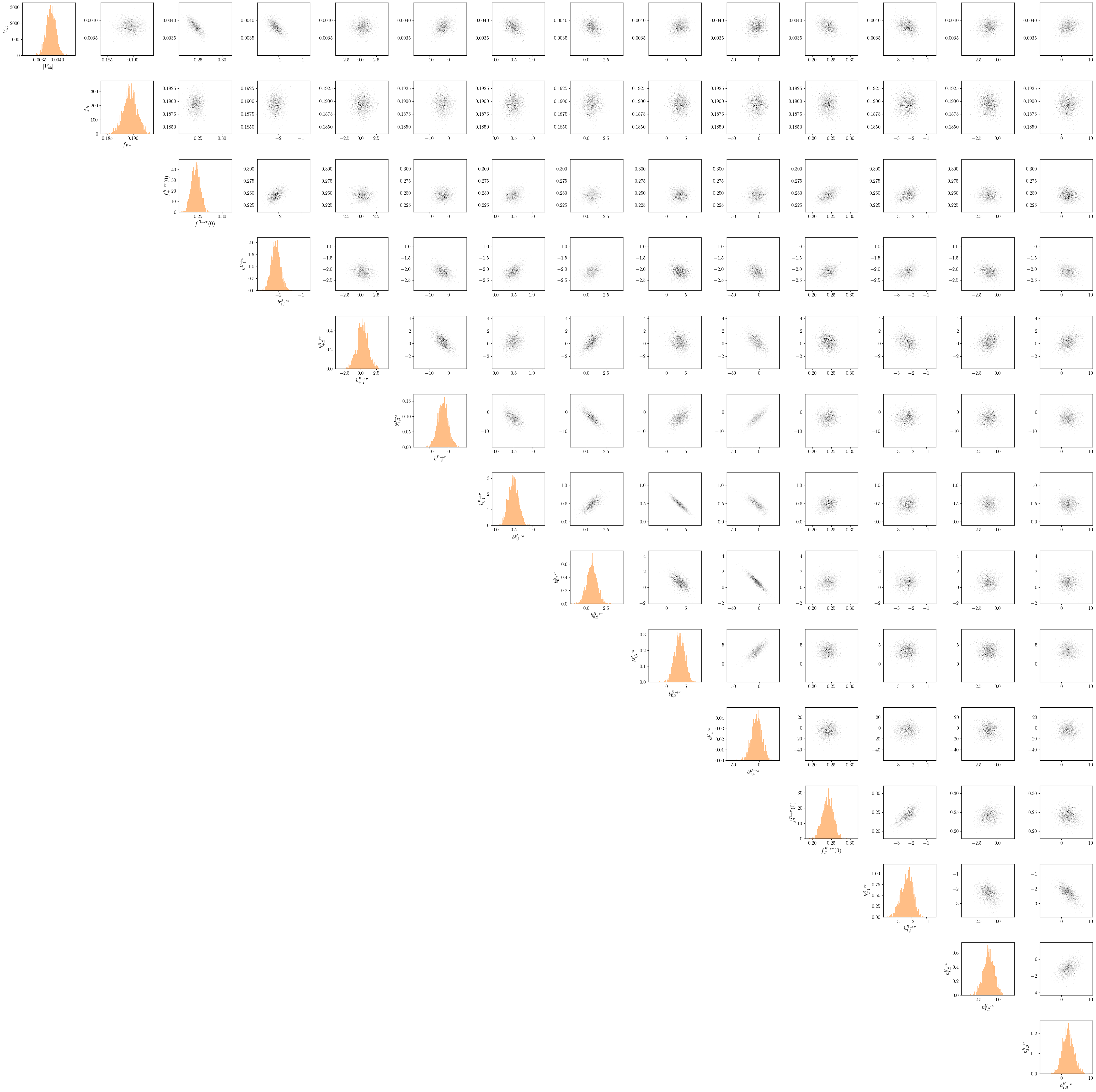
Finally, we can visualize our results using the corner_plot task:

eos.tasks.corner_plot(analysis_file=af, posterior='CKM-all', base_directory=BASE_DIRECTORY, format=['pdf', 'png'])

To repeat this process for the WET-all posterior, we simply specify this in the task:

af = eos.AnalysisFile('./b-to-u-l-nu.yaml')

eos.tasks.sample_nested(af, 'WET-all', base_directory=BASE_DIRECTORY, bound='multi', nlive=100, dlogz=9.0, maxiter=4000)

[ObservableEntries.insert_or_assign] Entry for observable B->pilnu::R_pi has been replaced.

We can access our results using the eos.data module, as above:

path = os.path.join(BASE_DIRECTORY, 'WET-all', 'nested')
ns_results = eos.data.DynestyResults(path)

# Obtain dynesty results object
dyn_results = ns_results.results
# this can be used, for example, for a quick summary
dyn_results.summary()

Summary
=======
niter: 4065
ncall: 117370
eff(%):  3.104
logz: 224.641 +/-  0.373

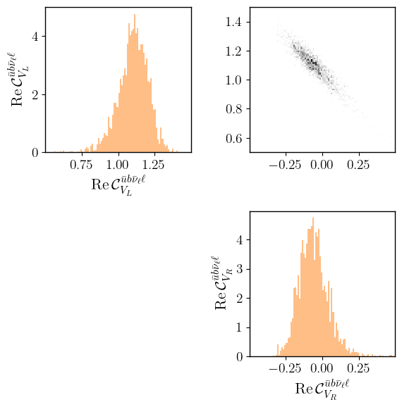
We can plot only part of the posterior by passing the start and end arguments to eos.tasks.corner_plot. Here we plot a marginal posterior for the Wilson coefficients.

eos.tasks.corner_plot(analysis_file=af, posterior='WET-all', base_directory=BASE_DIRECTORY, format=['pdf', 'png'], end=2)

We can also generate posterior-predictive samples. Here we produce samples for the branching ratio of the leptonic decay \(\bar{B} \to \ell^- \bar{\nu}\):

eos.tasks.predict_observables(
    analysis_file=af, posterior='CKM-all',
    prediction='leptonic-BR-CKM',
    base_directory=BASE_DIRECTORY
    )

These samples can be analyzed as described in the inference notebook, e.g. with:

predictions = eos.data.Prediction('./CKM-all/pred-leptonic-BR-CKM')
lo, mi, up = eos.Plotter._weighted_quantiles(
        predictions.samples[:, 0], # Here 0 gives access to the prediction with the option l = e
        [0.15865, 0.5, 0.84135],
        predictions.weights
        )

md(f"""$\\mathcal{{B}}(\\bar{{B}} \\to e^- \\bar{{\\nu}}_e) = \
        {10**12*mi:.2f} ^ {{+{10**12*(up-mi):.2f}}} _ {{{10**12*(lo-mi):.2f}}} \\times 10^{{-12}}$
        (from a naive sampling)""")

\(\mathcal{B}(\bar{B} \to e^- \bar{\nu}_e) = 9.82 ^ {+0.74} _ {-0.69} \times 10^{-12}\) (from a naive sampling)

Similarly, for the WET-all posterior:

eos.tasks.predict_observables(
    analysis_file=af, posterior='WET-all',
    prediction='leptonic-BR-WET',
    base_directory=BASE_DIRECTORY
    )

predictions = eos.data.Prediction('./WET-all/pred-leptonic-BR-WET')
lo, mi, up = eos.Plotter._weighted_quantiles(
        predictions.samples[:, 0], # Here 0 gives access to the prediction with the option l = e
        [0.15865, 0.5, 0.84135],
        predictions.weights
        )

md(f"""$\\mathcal{{B}}(\\bar{{B}} \\to e^- \\bar{{\\nu}}_e) = \
        {10**12*mi:.2f} ^ {{+{10**12*(up-mi):.2f}}} _ {{{10**12*(lo-mi):.2f}}} \\times 10^{{-12}}$
        (from a naive sampling)""")

\(\mathcal{B}(\bar{B} \to e^- \bar{\nu}_e) = 12.42 ^ {+4.06} _ {-3.89} \times 10^{-12}\) (from a naive sampling)

Lastly, we can also make a prediction for our custom R_pi observable. Since this observable is constructed as the ratio of two branching ratios, which have the same functional form and parameter dependence, the uncertainties cancel almost exactly.

eos.tasks.predict_observables(
    analysis_file=af, posterior='CKM-all',
    prediction='R_pi',
    base_directory=BASE_DIRECTORY
    )

predictions = eos.data.Prediction('./CKM-all/pred-R_pi')
lo, mi, up = eos.Plotter._weighted_quantiles(
        predictions.samples[:, 0], # Here 0 gives access to the prediction with the option l = e
        [0.15865, 0.5, 0.84135],
        predictions.weights
        )

md(f"""$\\mathcal{{R}}_\pi = \
        {mi:.2g} ^ {{+{(up-mi):.2g}}} _ {{{(lo-mi):.2g}}}$
        (from a naive sampling)""")

\(\mathcal{R}_\pi = 0.74 ^ {+1.1e-16} _ {-1.1e-16}\) (from a naive sampling)