Parameter Inference
EOS can infer parameters based on a database of experimental or theoretical constraints and its built-in observables. The examples in this notebook illustrate how to find a specific constraint from the list of all built-in observables, include them in an analysis file, and infer mean value and standard deviation of a list of parameters through sampling methods.
[1]:
import eos
import numpy as np
Listing the built-in Constraints
The full list of built-in constraints for the most-recent EOS release is available online here. You can also show this list using the eos.Constraints class. Searching for a specific constraint is possible by filtering for specific strings in the constraint name’s prefix, name, or suffix parts. The following example only shows constraints that contain a '->D' in the prefix part:
[2]:
eos.Constraints(prefix='B^0->D^+')
[2]:
| qualified name | observables | type | reference |
|---|---|---|---|
| B^0->D^+e^-nu::BRs@Belle:2015A | ... | MultivariateGaussian(Covariance) | Belle:2015A |
| B^0->D^+l^-nu::KinematicalDistribution[w]@Belle:2015A | ... | MultivariateGaussian(Covariance) | Belle:2015A |
| B^0->D^+mu^-nu::BRs@Belle:2015A | ... | MultivariateGaussian(Covariance) | Belle:2015A |
Visualizing the built-in Constraints
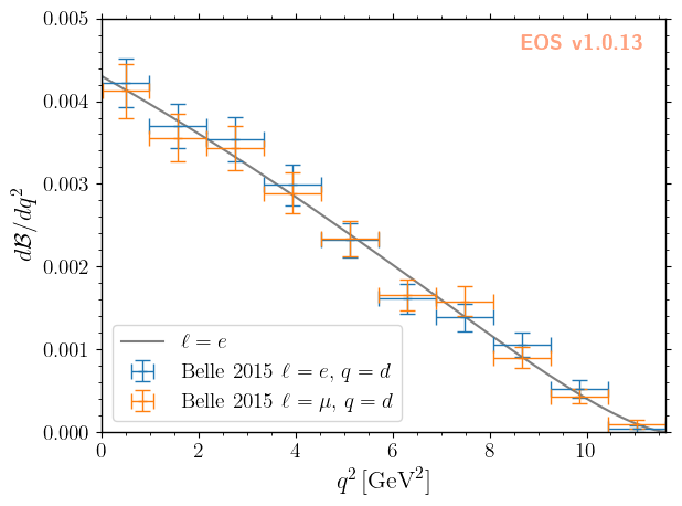
For what follows we will use the two experimental constraints B^0->D^+e^-nu::BRs@Belle:2015A and B^0->D^+mu^-nu::BRs@Belle:2015A, to infer the CKM matrix element \(|V_{cb}|\). We can readily display these two constraints, along with the default theory prediction (without any uncertainties), using the following code:
[3]:
plot_args = {
    'plot': {
        'x': { 'label': r'$q^2$', 'unit': r'$\textnormal{GeV}^2$', 'range': [0.0, 11.63] },
        'y': { 'label': r'$d\mathcal{B}/dq^2$',                    'range': [0.0,  5e-3] },
        'legend': { 'location': 'lower left' }
    },
    'contents': [
        {
            'label': r'$\ell=e$',
            'type': 'observable',
            'observable': 'B->Dlnu::dBR/dq2;l=e,q=d',
            'variable': 'q2',
            'color': 'black',
            'range': [0.02, 11.63],
        },
        {
            'label': r'Belle 2015 $\ell=e,\, q=d$',
            'type': 'constraint',
            'color': 'C0',
            'constraints': 'B^0->D^+e^-nu::BRs@Belle:2015A',
            'observable': 'B->Dlnu::BR',
            'variable': 'q2',
            'rescale-by-width': True
        },
        {
            'label': r'Belle 2015 $\ell=\mu,\,q=d$',
            'type': 'constraint',
            'color': 'C1',
            'constraints': 'B^0->D^+mu^-nu::BRs@Belle:2015A',
            'observable': 'B->Dlnu::BR',
            'variable': 'q2',
            'rescale-by-width': True
        },
    ]
}
_ = eos.plot.Plotter(plot_args).plot()
Defining the analysis
To define our statistical analysis for the inference of \(|V_{cb}|\) from measurements of the \(\bar{B}\to D\ell^-\bar\nu\) branching ratios, we must decide how to parametrize the hadronic form factors that emerge in semileptonic \(\bar{B}\to D\) transitions and how to constraint them. On top of the theoretical constraints and form factor coefficient priors as in predictions.yaml, we must add a prior for varying the CKM element and experimental constraints from which to extract
it. We only vary the absolute value of the CKM element CKM::abs(V_cb), as the complex phase of the CKM element CKM::arg(V_cb) is not accessible from \(b\to c \ell \bar \nu\). In order to use this parametrization of the CKM elements, we must use the model CKM in the analysis.
These additions to the likelihood and priors, seen in the analysis file inference.yaml, look like
priors:
  - name: CKM
    descriptions:
      - { parameter: 'CKM::abs(V_cb)',           min:  38e-3, max:  45e-3 , type: 'uniform' }

  - name: FF
    # as in both predictions.yaml and inference.yaml

likelihoods:
  - name: B-to-D-l-nu
    constraints:
      - 'B^0->D^+e^-nu::BRs@Belle:2015A;form-factors=BSZ2015'
      - 'B^0->D^+mu^-nu::BRs@Belle:2015A;form-factors=BSZ2015'

  - name: FF-LQCD
    # as in both predictions.yaml and inference.yaml
Sampling from the posterior
EOS provides the means to draw and store Monte Carlo samples for a prior PDF \(P_0(\vec\vartheta)\), a posterior PDF \(P(\vec\vartheta|\text{data})\), and predictive distributions using eos.tasks.sample_nested. We store this data within a hierarchy of directories below a “base directory”. For the purpose of the following examples, we set this base directory to ./inference-data, stored in a convenient global variable.
[4]:
EOS_BASE_DIRECTORY='./inference-data'
[5]:
eos.tasks.sample_nested('inference.yaml', 'CKM', base_directory=EOS_BASE_DIRECTORY, nlive=250, dlogz=0.5, seed=42)
Inferring the \(|V_{cb}|\) parameter
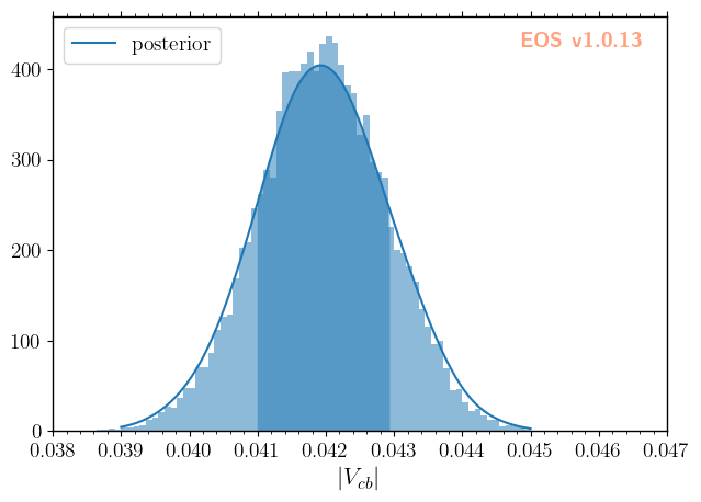
The distribution of the parameter samples, here using \(|V_{cb}|\) as an example, can be inspected using regular histograms or a smooth histogram based on a kernel density estimate (KDE). The samples are automatically processed, when specifying the data-file directory and the variable as histogram plotting arguments. For the KDE, the parameter bandwidth regulates the smoothing. EOS applies a relative bandwidth factor with respect to SciPy’s best bandwidth estimate, i.e.,
specifying 'bandwidth': 2 doubles SciPy’s estimate for the bandwidth.
[6]:
plot_args = {
    'plot': {
        'x': { 'label': r'$|V_{cb}|$', 'range': [38e-3, 47e-3] },
        'legend': { 'location': 'upper left' }
    },
    'contents': [
        {
            'type': 'histogram',
            'variable': 'CKM::abs(V_cb)',
            'data-file': EOS_BASE_DIRECTORY+'/CKM/samples'
        },
        {
            'type': 'kde', 'color': 'C0', 'label': 'posterior', 'bandwidth': 2,
            'range': [39e-3, 45e-3],
            'variable': 'CKM::abs(V_cb)',
            'data-file': EOS_BASE_DIRECTORY+'/CKM/samples'
        }
    ]
}
_ = eos.plot.Plotter(plot_args).plot()
To extract further information from the parameter samples, we can load the sample values using eos.data.ImportanceSamples:
[7]:
parameter_samples = eos.data.ImportanceSamples(EOS_BASE_DIRECTORY+'/CKM/samples')
We can compute the mean value and its standard deviation using numpy methods, including the sample weights.
[8]:
mean = np.average(parameter_samples.samples[:,0], weights = parameter_samples.weights)
std = np.sqrt(np.average((parameter_samples.samples[:,0]-mean)**2, weights = parameter_samples.weights))

print(f'$|V_{{cb}}|$ = {mean:.4f} +/- {std:.4f}')
$|V_{cb}|$ = 0.0420 +/- 0.0009
We can also illustrate the correlation between \(|V_{cb}|\) and any form factor parameter. Here, we use the normalization of the form factors at \(q^2 = 0\) as an example. The data passed to the plotter consists of the 2d parameter samples and the corresponding sample weights. Contours of equal probability at the \(68\%\) and \(95\%\) levels can be generated using a KDE as follows:
[9]:
plot_args = {
    'plot': {
        'x': { 'label': r'$|V_{cb}|$', 'range': [38e-3, 47e-3] },
        'y': { 'label': r'$f_+(0)$',   'range': [0.6, 0.75] },
    },
    'contents': [
        {
            'type': 'kde2D', 'color': 'C1', 'label': 'posterior',
            'levels': [68, 95], 'contours': ['lines','areas'], 'bandwidth':3,
            'data': {
                'samples': parameter_samples.samples[:, (0,1)],
                'weights': parameter_samples.weights
            }
        }
    ]
}
_ = eos.plot.Plotter(plot_args).plot()
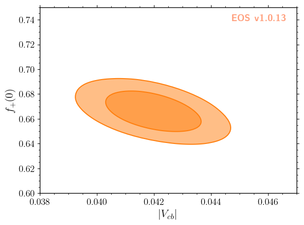
Here the bandwidth parameter takes the same role as in the 1D histogram.
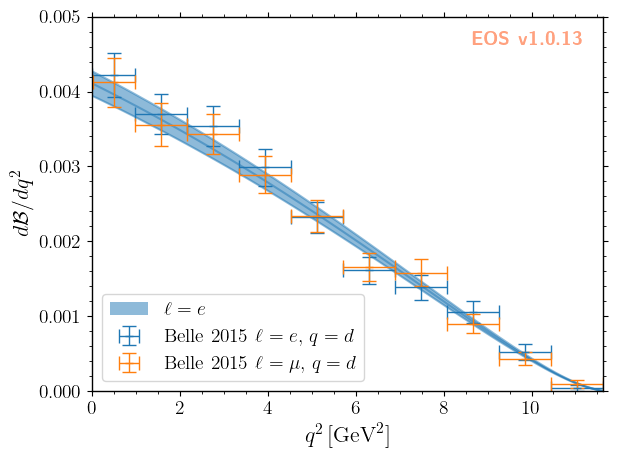
Aside: validating the posterior
As an additional step we can visualize the resulting theory prediction (with uncertainties), as was done in the beginning of this notebook. For further details, you can consult the predictions.ipynb notebook.
[10]:
eos.predict_observables('inference.yaml','CKM','B-to-D-e-nu', base_directory=EOS_BASE_DIRECTORY)
[11]:
plot_args = {
    'plot': {
        'x': { 'label': r'$q^2$', 'unit': r'$\textnormal{GeV}^2$', 'range': [0.0, 11.63] },
        'y': { 'label': r'$d\mathcal{B}/dq^2$',                    'range': [0.0,  5e-3] },
        'legend': { 'location': 'lower left' }
    },
    'contents': [
        {
          'label': r'$\ell=e$', 'type': 'uncertainty', 'range': [3.0e-7, 11.60],
          'data-file': EOS_BASE_DIRECTORY+'/CKM/pred-B-to-D-e-nu',
        },
        {
            'label': r'Belle 2015 $\ell=e,\, q=d$',
            'type': 'constraint',
            'color': 'C0',
            'constraints': 'B^0->D^+e^-nu::BRs@Belle:2015A',
            'observable': 'B->Dlnu::BR',
            'variable': 'q2',
            'rescale-by-width': True
        },
        {
            'label': r'Belle 2015 $\ell=\mu,\,q=d$',
            'type': 'constraint',
            'color': 'C1',
            'constraints': 'B^0->D^+mu^-nu::BRs@Belle:2015A',
            'observable': 'B->Dlnu::BR',
            'variable': 'q2',
            'rescale-by-width': True
        },
    ]
}
_ = eos.plot.Plotter(plot_args).plot()
[ ]: